Simple Markowitz Portfolio Optimzation Problem • rmpk

Here we solve a simple Markowitz Portfolio Optimization Problem. I really have no idea about security selection, but it is a good example of a continuous quadratic program.

The model

This example follows the formulation from here.

We have a number of \(n\) stocks. Each has an expected value of \(e_i\) and a covariance matrix \(C_{i,j}\). The question is now: can we construct a portfolio of stocks that gives us at least a return of \(\mu\) but with minimal variance? In order to do this we seek weights for our stocks that minimize the risk while giving us a lower bound on the expected return.

\[ \begin{equation*} \begin{array}{ll@{}ll} \text{min} & \displaystyle\sum\limits_{i=1}^{n}\sum\limits_{j=1}^{n}C_{i,j} \cdot x_{i} \cdot x_{j} & &\\ \text{subject to}& \displaystyle\sum\limits_{i=1}^{n} e_i \cdot x_{i} \geq \mu& &\\ & \displaystyle\sum\limits_{i=1}^{n} x_{i} = 1& & \\ & 0 \leq x_{i} \leq 1 &\forall i=1, \ldots, n & \end{array} \end{equation*} \]

In R

First we generate some data

set.seed(42)
n <- 10
returns <- matrix(
  rnorm(n * 20, 
        mean = runif(n, 0.01, 0.03), 
        sd = runif(n, 0.1, 0.4)), 
  ncol = n) # 20 time periods
# each col is a stock time series
e <- colMeans(returns)
C <- cov(returns)
min_mu <- 0.02

library(rmpk)
library(ROI.plugin.quadprog)

solver <- ROI_optimizer("quadprog")
model <- optimization_model(solver)
x <- model$add_variable("x", i = 1:n, lb = 0, ub = 1)
model$set_objective(sum_expr(2 * C[i, j] * x[i] * x[j], i = 1:n, j = 1:n))
model$add_constraint(sum_expr(e[i] * x[i], i = 1:n) >= min_mu)
model$add_constraint(sum_expr(x[i], i = 1:n) == 1)

model$optimize()

(results <- model$get_variable_value(x[i]))
#>    name  i         value
#> 1     x  1  4.656654e-02
#> 2     x  7  4.886324e-02
#> 3     x  5  7.361526e-02
#> 4     x  8  1.039045e-01
#> 5     x  2  3.285331e-18
#> 6     x 10  1.235237e-01
#> 7     x  9  2.243257e-01
#> 8     x  3  1.178596e-01
#> 9     x  6 -1.248999e-18
#> 10    x  4  2.613414e-01

library(ggplot2)
ggplot(results) + 
  aes(x = factor(i), y = value) + 
  geom_bar(stat = "identity", aes(fill = "Allocation")) + 
  geom_point(data = data.frame(i = factor(1:n), value = e), aes(color = "Expected return")) +
  xlab("Stocks") + 
  ylab("") +
  scale_fill_discrete() +
  scale_color_viridis_d() + 
  ggtitle("Optimal Portfolio")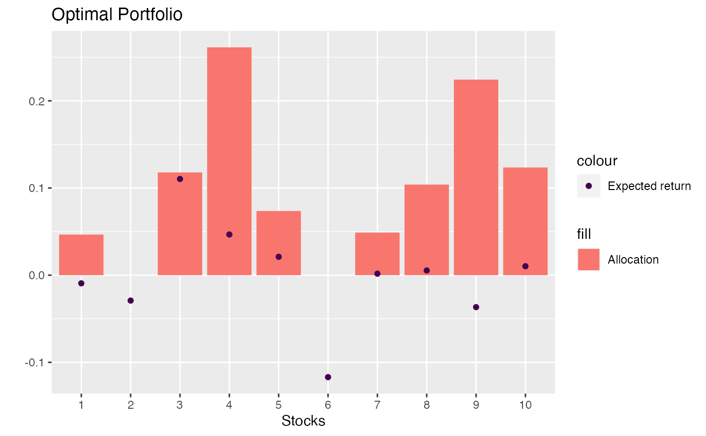

Bars are stock allocation and dots are the expected returns. It is a bit strange that the model allocates 20% of our portfolio to a stock with negative expected return - but maybe it reduces the volatility… or it is a bug :)

Feedback

Do you have any questions, ideas, comments? Or did you find a mistake? Let’s discuss on Github.